Metastable materials, phases that are kinetically trapped in an energetically unfavorable state, offer a tremendous playground to discover new compounds with fascinating properties. In the past, I was primarily studying pressure as a thermodynamic tuning knob to synthesize such metastable materials, and the recent discovery of the first quasi-room-temperature superconductor LaH10 has impressively demonstrated the capabilities of computation and simulation in the high-pressure community. Recently, however, I have switched my focus to investigating temperature as the main parameter to tune the synthesis condition in conjunction with rapid cooling (referred to as quenching) to trap metastable phases.

In particular, our team at Cornell uses lasers to locally and very quickly heat (referred to as anneal) thin films of amorphous materials deposited on silicon within temperatures between 300 and 1400°C. This technique is called laser spike annealing, or LSA in short. Most chemical systems exhibit several polymorphs in this temperature range, and with our experimental technique we can quickly map out what conditions and quench rates (or dwell times) lead to the formation of a specific phase.

Things get even more exciting when we include composition as an additional, tunable parameter: the thin films can be deposited as a composition gradient by co-depositing several elements from different spatial locations. In this way, we have complete control over temperature T, dwell time τ, and composition c to explore new phases in a high-throughput fashion.

Closing the loop

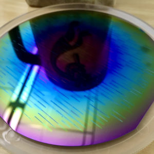
This large number of parameters however poses a new problem: the high dimension of our exploratory space renders its sampling very challenging. A single 100mm silicon wafer offers space for 625 laser anneal stripes, or in other words, we can choose 625 different conditions to perform our laser experiments. But how shall we choose these conditions? Of course we can create an equally spaced mesh in all parameter dimensions, e.g., 8x8x8 grid for temperature, dwell time, and composition, respectively. But this mesh is rather sparse, and might not even capture the most critical conditions, namely the phase boundaries, or the conditions at which one metastable phase forms and another disappears.

A laser spike annealed thin film sample. Every stripe corresponds to a specific laser condition used to perform an anneal experiment.

This is where computation and simulations become critically important: we can use machine learning to sample the parameter space intelligently, honing in on the conditions that are most interesting in terms of phase transitions. In particular, we use a specific kind of machine learning, called active learning: after performing an LSA experiment, we analyze the results and simulate the phase boundaries, and based on the outcome decide which condition to sample next: we learn the phase map on the fly by selecting conditions most valuable for our model to become more accurate. This loop is repeated, and as we keep adding more and more data to our model, the predicted synthesis conditions for a specific phase becomes better and better. Our ultimate goal is to create a framework, essentially a robot, that can autonomously explore the complete synthesis phase diagram of any system using this machine learning method, a feat that we call “closing the loop”.

A picture says more than words

But how do we determine what condition leads to the formation of which phase? The ultimate experimental analysis technique for this purpose is x-ray diffraction (XRD), which essentially creates a picture of the electron distribution in a crystal lattice, and can be converted back into a model of the atomic arrangement in a crystal structure. Sufficiently accurate XRD measurements for our samples can only be performed with so-called synchrotron radiation, where the Bremsstrahlung emitted by particles going in a large circle produce highly coherent and extremely intense x-rays. Unfortunately, access to such synchrotron experiments is very limited, providing us only a window of a few days per year to perform our XRD characterizations.

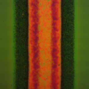
A microscopy image of a laser spike annealed region of bismuth oxide on a silicon wafer. Note that the stripe is symmetric about the y-axis, since the power profile resembles a Gaussian distribution with the peak power at its center.

To circumvent this issues, we have developed a new, more accessible method to assess the phase boundaries, namely by relying on optical data only. In short, we learned how to use (fancy) photographs of our samples to determine the phase boundaries in our active learning loop without having to perform a single XRD experiment. Nevertheless, x-rays are still needed as the ultimate method to confirm our predictions.

Yesterday, our team wrapped up a 5-day long beam time at the Cornell High Energy Synchrotron Source (CHESS), where we collected XRD data for our LSA annealed samples of various chemical systems. The weeks leading up to the XRD experiment, and the CHESS run itself, were intense, and we worked around the clock to overcome unexpected setbacks and to assemble the required software and hardware infrastructure. As I am writing this article I am on my way home for the holidays, and I am excited to announce that we have indeed successfully closed the loop!